선형 회귀(Linear Regression)

선형 회귀(Linear Regression)는 지도학습(Supervised Learning)의 일종으로 단순 선형 회귀(Simple)와 다중 선형 회귀(Multiple)가 있습니다.

선형 회귀는 선형이라는 이름에 맞게 일차원 함수의 형태로 나타납니다. 

 

단순 선형 회귀(Simple Linear Regression)

단순 선형 회귀는 하나의 종속변수(Dependent Variable)와 하나의 독립변수(Independent Variable) 사이의 관계를 모델링 하는 기법입니다.

이걸 Tensorflow를 이용하여 구현하며 알아보도록 하겠습니다.

일단 선형 회귀를 하기 위해선 데이터가 필요합니다.

y = 2x + 3을 기준으로 랜덤한 값을 더해서 데이터를 만들어 보겠습니다.

import tensorflow as tf
import matplotlib.pyplot as plt
import numpy as np

@tf.function
def f(x):
    y = 2 * x + 3
    return y

x = tf.linspace(0, 5, 101)
x = tf.cast(x, tf.float32)
y = f(x) + tf.random.normal(shape=[101])

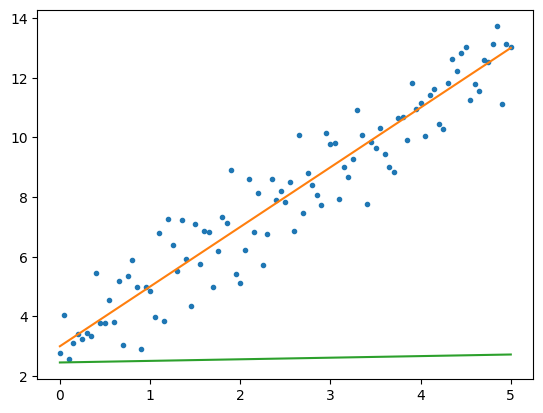
그리고 이 데이터를 예측할 모델과 가설(Hypothesis)를 만들어 보겠습니다.

class Model(tf.Module):
    def __init__(self, seed=22):
        rand_init = tf.random.uniform(shape=[2], minval=0., maxval=5., seed=seed)

        self.w = tf.Variable(rand_init[0])
        self.b = tf.Variable(rand_init[1])
    
    @tf.function
    def __call__(self, x):
        y = self.w * x + self.b
        return y

지금은 가중치(Weight, w)와 편향(Bias, b)를 랜덤값으로 초기화 해 뒀기 때문에 실제 값과 동떨어진 가설 그래프가 나올 것 입니다.

이제 이 그래프가 얼마나 실제 값과 동떨어져 있는지를 나타내주는 비용(Cost) 또는 손실(Loss)라 부르는 함수를 만들어 줄 것 입니다.

예측값과 실제값의 차를 구하기 위해서 주로 절대값을 이용하거나 제곱을 이용하는데, 제곱이 더 계산하기 편하기 때문에 제곱을 이용한 평균 제곱 오차(Mean Squared Error)라는 방식을 사용할 것 입니다.

def loss(y, y_pred):
    return tf.reduce_mean(tf.square(y - y_pred))

print(loss(y, model(x)))

tf.Tensor(37.40411, shape=(), dtype=float32)

37.40411이 예측값과 실제값을 손실함수에 넣어서 나온 결과입니다.

from mpl_toolkits.mplot3d import Axes3D
from tqdm import tqdm

ax = plt.subplot(111, projection='3d')

w = np.linspace(0, 5, 101)
b = np.linspace(0, 5, 101)

W, B = np.meshgrid(w, b)

Z = np.zeros(shape=[101, 101])

pbar = tqdm(total=101*101)
for i in range(101):
    for j in range(101):
        model = Model()
        model.w = W[i, j]
        model.b = B[i, j]
        Z[i, j] = loss(y, model(x))
        pbar.update(1)

ax.plot_surface(W, B, Z, cmap='viridis')
ax.set_xlabel('w')
ax.set_ylabel('b')
ax.set_zlabel('loss')

그래프 이미지가 조금 잘리긴 했지만 대충 어느 정도에서 loss함수가 최소값을 갖는지 알아볼 수 있습니다.

이제 가설 함수의 가중치와 편향을 조정해 loss를 최소로 만들어야 하는데 이를 해주는 알고리즘이 Optimizer라 불리는 경사하강법, Adam등의 것들 입니다.

model = Model()

with tf.GradientTape() as tape:
    tape.watch(model.variables)
    loss_v = loss(y, model(x))
print(tape.gradient(loss_v, model.variables))

tensorflow에서는 자동 미분을 지원해주기 때문에 위와 같이 코드를 작성하면 각각의 편미분값을 알 수 있습니다.

하지만 w와 b가 랜덤인 상태이기 때문에 값이 랜덤하게 나올것입니다.

경사하강법에 따라 미분값과 learning rate를 곱하여 각 변수에서 빼주면 됩니다.

epochs = 100
learning_rate = 0.01

model = Model()

with tf.GradientTape() as tape:
    tape.watch(model.variables)
    batch_loss = loss(y, model(x))
grad = tape.gradient(batch_loss, model.variables)
print(grad)
model.w.assign_sub(learning_rate * grad[0])
model.b.assign_sub(learning_rate * grad[1])

with tf.GradientTape() as tape:
    tape.watch(model.variables)
    batch_loss = loss(y, model(x))
grad = tape.gradient(batch_loss, model.variables)
print(grad)
model.w.assign_sub(learning_rate * grad[0])
model.b.assign_sub(learning_rate * grad[1])

with tf.GradientTape() as tape:
    tape.watch(model.variables)
    batch_loss = loss(y, model(x))
print(tape.gradient(batch_loss, model.variables))

(<tf.Tensor: shape=(), dtype=float32, numpy=-5.1804476>, <tf.Tensor: shape=(), dtype=float32, numpy=-12.510265>)
(<tf.Tensor: shape=(), dtype=float32, numpy=-4.671219>, <tf.Tensor: shape=(), dtype=float32, numpy=-11.017024>)
(<tf.Tensor: shape=(), dtype=float32, numpy=-4.217317>, <tf.Tensor: shape=(), dtype=float32, numpy=-9.6837435>)

몇번 돌려보게 되면 미분값이 점점 0에 근접해간다는걸 알 수 있습니다.

이걸 한 100번정도 돌리게 되면 loss를 거의 최소로 만들 수 있습니다.

epochs = 100
learning_rate = 0.01
losses = []

model = Model()

for epoch in range(epochs):
    with tf.GradientTape() as tape:
        tape.watch(model.variables)
        batch_loss = loss(y, model(x))
    grads = tape.gradient(batch_loss, model.variables)
    for g,v in zip(grads, model.variables):
        v.assign_sub(learning_rate*g)

    loss_v = loss(y, model(x))
    losses.append(loss_v)
    if epoch % 10 == 0:
        print(f'Loss of step {epoch}: {loss_v.numpy():0.3f}')

plt.plot(range(epochs), losses)
plt.xlabel("Epoch")
plt.ylabel("Loss (MSE)")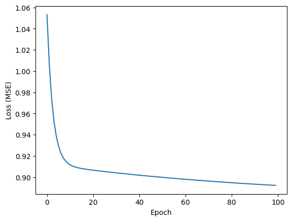

학습된 결과를 그래프로 찍어보겠습니다.

plt.figure()
plt.plot(x, y, '.')
plt.plot(x, f(x))
plt.plot(x, model(x))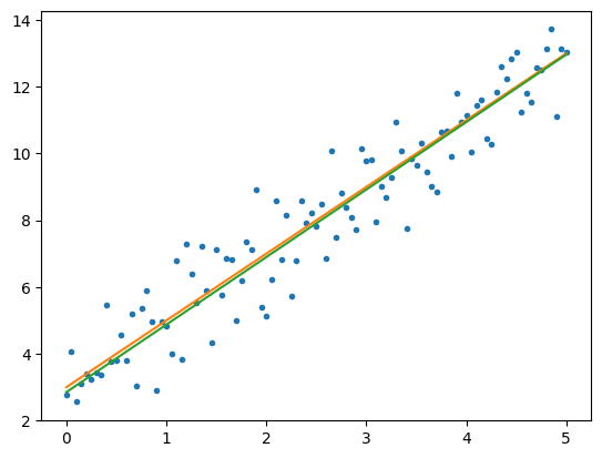

그리고 원본 그래프와 loss 를 비교해 보겠습니다.

print(loss(y, model(x)))
print(loss(y, f(x)))

tf.Tensor(0.89216924, shape=(), dtype=float32)
tf.Tensor(0.8852339, shape=(), dtype=float32)

0.89216924와 0.8852339로 학습된 모델의 loss가 약간 더 크긴 하지만 학습이 잘 됐다고 볼 수 있겠습니다.

SimpleLinearRegression.ipynb

0.22MB

다중 선형 회귀(Multiple Linear Regression)

import tensorflow as tf
import matplotlib.pyplot as plt
from mpl_toolkits.mplot3d import Axes3D
import numpy as np

@tf.function
def f(x, y):
    z = 2 * x + y + 3
    return z

x = tf.linspace(0, 5, 101)
x = tf.cast(x, tf.float32)
y = tf.linspace(0, 5, 101)
y = tf.cast(y, tf.float32)

z = f(x, y) + tf.random.normal(shape=[101])

fig = plt.figure()
ax = fig.add_subplot(111, projection='3d')
ax.scatter(x, y, z, c='r', marker='o')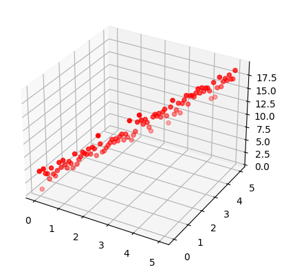

class Model(tf.Module):
    def __init__(self, seed=22):
        rand_init = tf.random.uniform(shape=[3], minval=0., maxval=5., seed=seed)

        self.w_x = tf.Variable(rand_init[0])
        self.w_y = tf.Variable(rand_init[1])
        self.b = tf.Variable(rand_init[2])
    
    @tf.function
    def __call__(self, x, y):
        z = self.w_x * x + self.w_y * y + self.b
        return z

model = Model()

fig = plt.figure()
ax = fig.add_subplot(111, projection='3d')
ax.scatter(x, y, z, c='r', marker='o')
ax.plot3D(x, y, f(x, y), c='r')
ax.plot3D(x, y, model(x, y), c='b')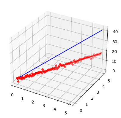

def loss(z, z_pred):
    return tf.reduce_mean(tf.square(z - z_pred))

print(loss(z, model(x, y)))

tf.Tensor(194.73457, shape=(), dtype=float32)

epochs = 100
learning_rate = 0.01

model = Model()

with tf.GradientTape() as tape:
    tape.watch(model.variables)
    batch_loss = loss(z, model(x, y))
grads = tape.gradient(batch_loss, model.variables)
print(grads)
for g,v in zip(grads, model.variables):
    v.assign_sub(learning_rate*g)

with tf.GradientTape() as tape:
    tape.watch(model.variables)
    batch_loss = loss(z, model(x, y))
grads = tape.gradient(batch_loss, model.variables)
print(grads)
for g,v in zip(grads, model.variables):
    v.assign_sub(learning_rate*g)

with tf.GradientTape() as tape:
    tape.watch(model.variables)
    batch_loss = loss(z, model(x, y))
print(tape.gradient(batch_loss, model.variables))

(<tf.Tensor: shape=(), dtype=float32, numpy=-12.747607>, <tf.Tensor: shape=(), dtype=float32, numpy=-38.576015>, <tf.Tensor: shape=(), dtype=float32, numpy=-38.576015>)
(<tf.Tensor: shape=(), dtype=float32, numpy=-8.635053>, <tf.Tensor: shape=(), dtype=float32, numpy=-25.01567>, <tf.Tensor: shape=(), dtype=float32, numpy=-25.01567>)
(<tf.Tensor: shape=(), dtype=float32, numpy=-5.9607844>, <tf.Tensor: shape=(), dtype=float32, numpy=-16.203669>, <tf.Tensor: shape=(), dtype=float32, numpy=-16.203669>)

epochs = 1000
learning_rate = 0.01
losses = []

model = Model()

for epoch in range(epochs):
    with tf.GradientTape() as tape:
        tape.watch(model.variables)
        batch_loss = loss(z, model(x, y))
    grads = tape.gradient(batch_loss, model.variables)
    for g,v in zip(grads, model.variables):
        v.assign_sub(learning_rate*g)

    loss_v = loss(z, model(x,y ))
    losses.append(loss_v)
    if epoch % 10 == 0:
        print(f'Loss of step {epoch}: {loss_v.numpy():0.3f}')

plt.plot(range(epochs), losses)
plt.xlabel("Epoch")
plt.ylabel("Loss (MSE)")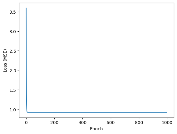

fig = plt.figure()
ax = fig.add_subplot(111, projection='3d')
ax.scatter(x, y, z, c='r', marker='o')
ax.plot3D(x, y, f(x, y), c='r')
ax.plot3D(x, y, model(x, y), c='b')

print(loss(z, model(x, y)))
print(loss(z, f(x,y )))

tf.Tensor(0.9223384, shape=(), dtype=float32)
tf.Tensor(0.9513635, shape=(), dtype=float32)

MultipleLinearRegression.ipynb

0.26MB